[Paper Review] Deep inside Convolutional networks Visualising Image Classification Models and Saliency Maps
[Paper Review] Deep inside Convolutional networks Visualising Image Classification Models and Saliency Maps
주요 contribution
- 이전 연구와 달리 supervised 방식으로 학습한 모델을 시각화
- 주어진 이미지 대해서 특정 클래스의 spatial support 계산 (image-specific class saliency map)
- gradient 기반의 시각화 방법과 deconvolutional network reconstruction 사이의 관계를 정립
Class model visualization
- 학습이 완료된 CNN 분류 모델이 주어졌을 때, 클래스를 대표하는 이미지 $I$를 생성 (image-specific X)
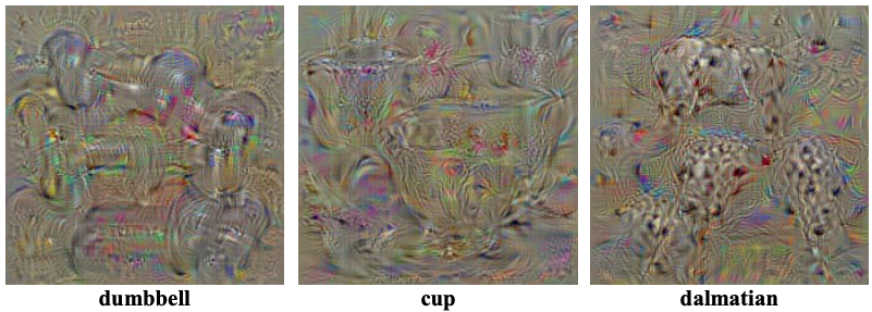
- 모든 클래스에 대해서 아래의 과정을 수행
Step 1zero-centered 이미지를 랜덤하게 생성해서 이미지 $I$를 초기화1
self.created_image = np.uint8(np.random.uniform(0, 255, (224, 224, 3)))
Step 2입력 이미지를 convolutional network로 학습Step 3class score $S_c$ 구하기- softmax layer의 output인 class posterior $P_c=\frac{expS_c}{\sum_cexpS_c}$가 아니라 정규화되지 않은 class score $S_c$를 사용
- $P_c$를 최대화하려면 다른 class의 $S_c$를 최소화해야 하지만, $S_c$를 최적화하면 최적화 대상인 특정 class에 집중할 수 있음
Step 4weight를 고정시키고, loss를 이미지 $I$에 대해 미분해서 이미지 $I$를 업데이트- objective function
- loss function
objective function에 L2 norm term을 사용하는 이유? 이 과정의 목적은 class score를 최대화하는 이미지 $I$를 찾는 것인데, L2 regularization을 사용하면 이미지 $I$의 픽셀 값이 너무 큰 값을 갖지 않도록 학습되기 때문에 (큰 값을 갖는 픽셀의 개수가 적기 때문에) 클래스의 특징이 비교적 잘 보임 (관련 링크)
norm term X (너무 밝다) L1 norm (너무 어둡다) L2 norm (잘 보인다!) 

Step 52~4를 반복1 2 3 4 5 6 7 8 9 10 11 12 13 14 15 16 17 18 19 20 21 22 23 24 25 26 27 28 29 30 31 32 33 34 35 36
def generate(self, iterations=150): """Generates class specific image Keyword Arguments: iterations {int} -- Total iterations for gradient ascent (default: {150}) Returns: np.ndarray -- Final maximally activated class image """ initial_learning_rate = 6 for i in range(1, iterations): # Process image and return variable self.processed_image = preprocess_image(self.created_image, False) # Define optimizer for the image optimizer = SGD([**self.processed_image**], lr=initial_learning_rate) # Forward output = self.model(self.processed_image) # Target specific class **class_loss = -output[0, self.target_class]** if i % 10 == 0 or i == iterations-1: print('Iteration:', str(i), 'Loss', "{0:.2f}".format(class_loss.data.numpy())) # Zero grads self.model.zero_grad() # Backward class_loss.backward() # Update image optimizer.step() # Recreate image self.created_image = recreate_image(self.processed_image) if i % 10 == 0 or i == iterations-1: # Save image im_path = '../generated/class_'+str(self.target_class)+'/c_'+str(self.target_class)+'_'+'iter_'+str(i)+'.jpg' save_image(self.created_image, im_path) return self.processed_image
Image-Specific Class Saliency Visualisation
- 주어진 이미지에 대해서 특정 클래스에 대해 spatial support 계산
- 클래스에 대한 영향력에 따라 이미지 픽셀들에 순위를 매김
이미지 $I_0$가 주어졌을 때, class score $S_c$ 를 이미지 $I$에 대해 미분한 값의 크기는 class score에 가장 큰 영향을 미치기 위해 어떤 픽셀이 가장 적게 변경되어야 하는지(=어떤 픽셀들이 object location에 해당하는지) 나타냄
\[w=\frac{\partial S_c}{\partial I}\bigg|_{I_0}\]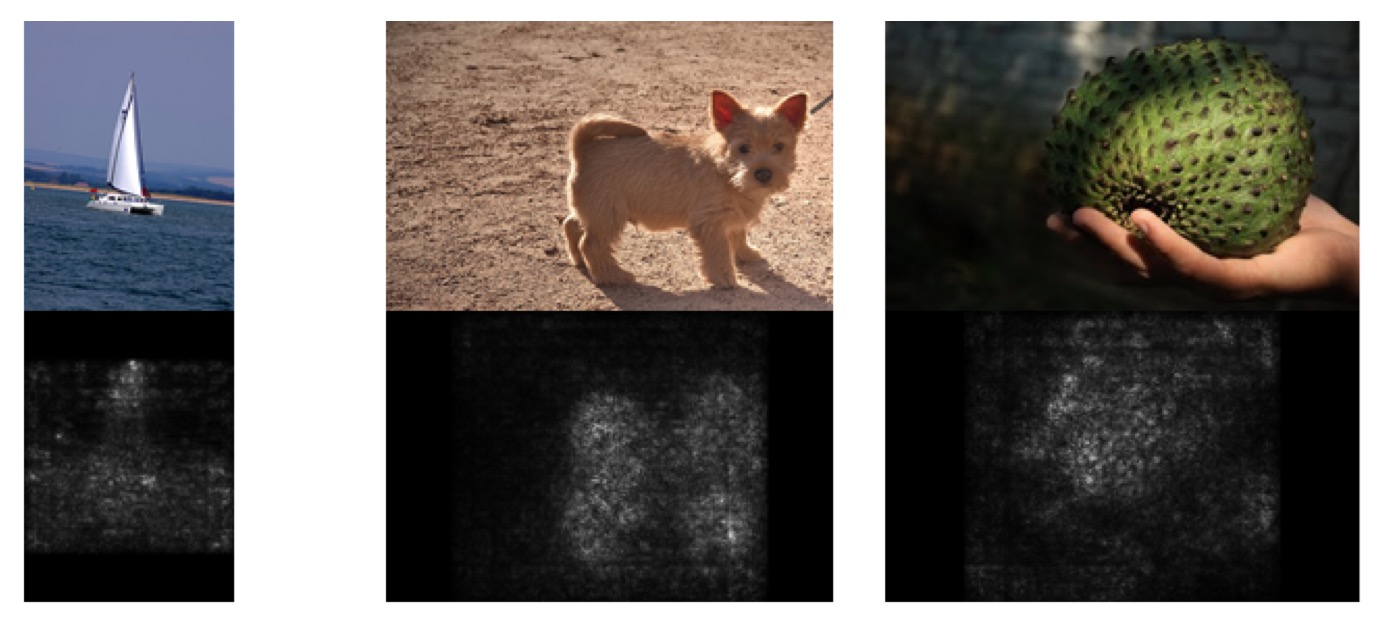
Class Saliency Extraction
$m$개의 row와 $n$개의 column으로 이루어진 이미지 $I_0$가 주어졌을 때, back-propagation을 통해 얻어지는 class saliency map $M$의 사이즈는 이미지 $I_0$의 사이즈와 동일함
\[M \in R^{m \times n}\]이미지가 흑백인 경우
\[M_{ij}=|w_{h(i,j)}|\]이미지가 컬러인 경우, 각 픽셀의 채널 값들 중 최댓값을 취함
\[M_{ij}=\max{|w_{h(i,j,c)}|}\]
Weakly Supervised Object Localisation
GraphCut
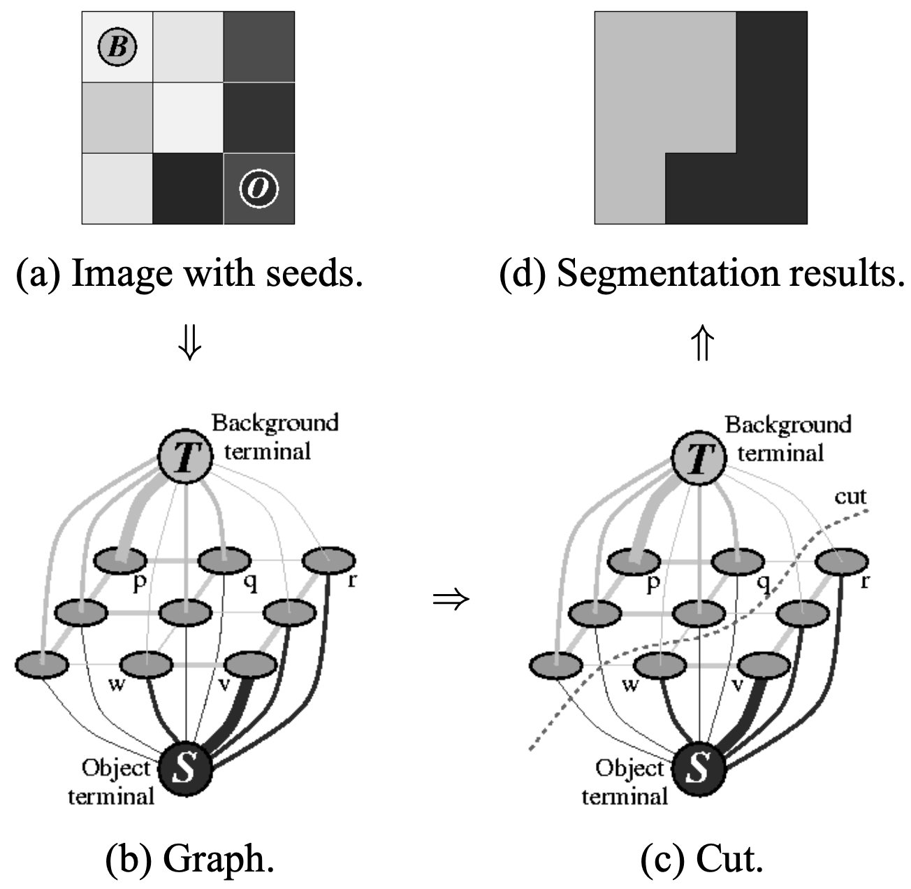
- GraphCut은 graph 상에서 loss를 최소화하는(=background 그룹과 object 그룹을 잘 구분짓는) 지점을 찾아서 cut 하는 알고리즘 (관련 논문, 참고하면 좋은 강의)
- 픽셀 간 차이가 큰데 라벨이 동일하거나 픽셀 간 차이가 작은데 라벨이 다르면 loss가 증가함. 예를 들어, 위에서 그림 (a)의 두 픽셀 (0,0), (0,1)은 픽셀 값 차이가 거의 없으므로 같은 라벨이어야 작은 loss를 가짐. 반대로, (0,1)과 (0,2)는 픽셀 값 차이가 크기 때문에 다른 라벨이어야 작은 loss를 가짐.
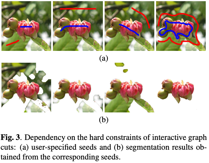
- 최초에 사용자가 seed를 설정하는 과정이 필요하고(그림 (a)처럼 대략적으로 어떤 부분이 object 또는 background인지), seed를 어떻게 설정하느냐에 따라서 segmentation quality가 좌우됨 (아래 이미지)
saliency map을 이용한 graph cut
- saliency map은 어떤 object를 다른 클래스와 구분 가능하게 하는 특징적인 부분만을 잡아내기 때문에 object 전체를 잡아낼 수 없음
- saliency map 값을 활용해 initial seed 설정 → GraphCut 알고리즘을 통해 특징적인 부분에서 이미지의 다른 부분으로 object의 경계를 확장
- saliency distribution에서 95% 이상의 값들(파란색)로부터 foreground 모델 추정
- saliency distribution에서 30% 이하의 값들(하늘색)로부터 background 모델 추정
- weakly supervised 방식임에도 불구하고 좋은 segmentation 성능을 보임
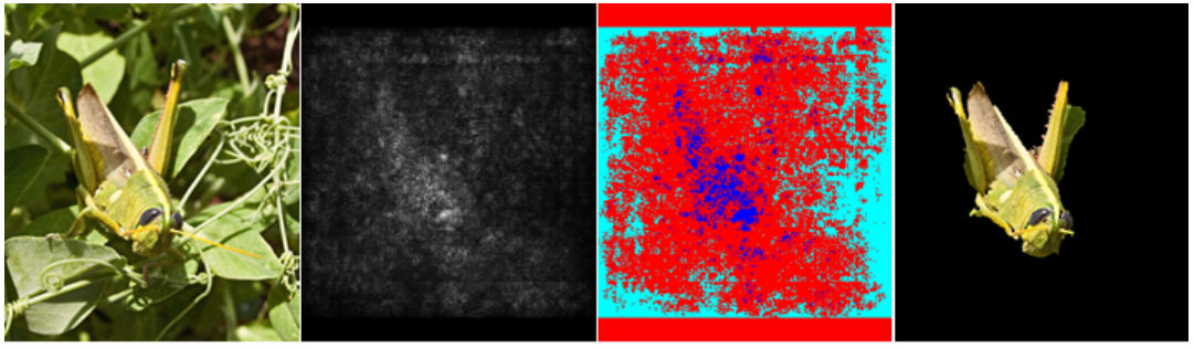
- 왼쪽부터 입력 이미지, saliency map, initial seed, segmentation 결과
Relation to Deconvolutional Networks
- gradient 기반 시각화 방법론과 deconvolutional network 구조 사이의 관계를 정립
- ConvNet에서
- $X_n$: $n$번째 layer의 입력값
- $K_n$: $n$번째 layer의 kernel
- $\hat{K_n}$: $n$번째 layer의 kernel의 flipped version 일 때,
\(X_{n+1} = X_{n} \star K_n\) \(X_n = X_{n+1} \star \hat{K_n}\)
- DeconvNet에서
- $R_n$: deconvolutional layer를 통해 복원된 $n$번째 feature map 일 때,
- 결국 DeconvNet을 통해 feature map을 복원하는 것과 $\frac{\partial f}{\partial X_n}$을 계산하는 것(gradient 기반 시각화)은 동일한 결과를 낳음
- gradient 기반 시각화 방법은 convolutional layer뿐만 아니라 network의 어떤 layer든 시각화할 수 있기 때문에 더 일반화된 방법이라고 볼 수 있음
- 본 논문에서는 마지막 fully-connected layer를 시각화
This post is licensed under CC BY 4.0 by the author.