[Paper Review] Swin Transformer: Hierarchical Vision Transformer using Shifted Windows

Posted Jan 25, 2023

By jieun choi 8 min read

Swin Transformer는 선행 연구인 Vision Transformer처럼 vision 분야에 Transformer 구조를 적용한 모델입니다. Swin Transformer를 소개하기에 앞서, Vision Transformer와의 주요 차이점을 살펴보면 다음과 같습니다. 논문을 리뷰해 보면서 아래 차이점들이 구체적으로 의미하는 바가 무엇인지 알아보겠습니다.

	Vision Transformer	Swin Transformer
self-attention 적용 방식	global self-attention	shifted window based self-attention
위치 정보 표현 방식	absolute position embedding	relative position bias
sliding window 적용 여부	$\times$	$\triangle$ (shifted window)

Introduction

Vision Transformer 이후에 vision 분야에 Transformer 구조를 적용하는 많은 논문이 발표되었는데요. language와 vision 도메인의 차이로 인해 vision 분야에 Transformer를 적용하기가 쉽지는 않았습니다.

첫 번째로, 고정된 크기를 가질 수 있는 language Transformer의 단어 토큰과 달리 시각적 요소들은 크기가 매우 다양합니다.
두 번째로, 텍스트를 구성하는 단어 토큰의 수보다 이미지를 구성하는 픽셀의 개수가 훨씬 많다는 것입니다. (=해상도가 매우 높음) 이 점은 sementic segmentation과 같이 픽셀 단위의 예측이 필요한 vision task에서 문제가 되는데요. self-attention을 수행할 때 연산 복잡도가 이미지 사이즈의 제곱에 비례하여 커지기 때문입니다.

위 한계점을 극복하기 위해 Swin Transformer는 hierarchical 구조와 window 안에서 local self-attention을 수행하는 방식을 적용했습니다. 이 때, 한 layer 안에서 self-attention을 수행하는 window들은 서로 겹치지 않습니다. 또 한가지 핵심 구조는 shifted window인데, Method 파트에서 좀 더 자세히 살펴보겠습니다.

Method

Swin Transformer 구조

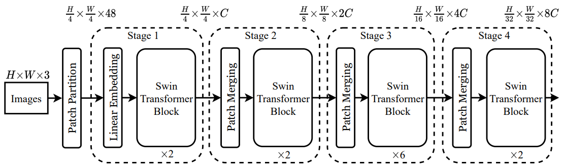
Swin Transformer가 입력 값을 처리하는 과정을 정리해보면 아래와 같습니다.

Step 1 [Patch Partition] RGB 채널을 갖는 입력 이미지 $x \in \mathbb{R}^{H \times W \times 3}$를 겹치지 않는 패치로 쪼개고, 각각의 패치를 NLP 문장의 token 처럼 사용합니다. 본 논문에서는 패치 사이즈로 $ 4 \times 4 $를 사용했으므로, 각 패치의 차원은 $ 4 \times 4 \times 3=48 $입니다.
Step 2 [Linear Embedding] 각각의 패치에 linear projection을 취해서 $C$차원에 매핑합니다.
Step 3 [Swin Transformer Block] $C$차원에 매핑한 패치를 Swin Transformer block에 입력합니다.
Step 4 [Patch Merging] $ 2 \times 2 $ 범위 내의 이웃 패치들을 합쳐 hierarchical representation을 생성합니다.
Step 5 [Swin Transformer Block] hierarchical representation을 Swin Transformer block에 입력합니다.
Step 6 [Patch Merging] $ 4 \times 4 $ 범위 내의 이웃 패치들을 합쳐 hierarchical representation을 생성합니다.
Step 7 [Swin Transformer Block] hierarchical representation을 Swin Transformer block에 입력합니다.
Step 8 [Patch Merging] $ 8 \times 8 $ 범위 내의 이웃 패치들을 합쳐 hierarchical representation을 생성합니다.
Step 9 [Swin Transformer Block] hierarchical representation을 Swin Transformer block에 입력합니다.
Step 10 [Patch Merging] $ 16 \times 16 $ 범위 내의 이웃 패치들을 합쳐 hierarchical representation을 생성합니다.
Step 11 마지막 hierarchical representation을 MLP head에 연결하여 classification을 수행합니다.

1. hierarchical representation 생성 과정

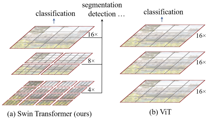Vision Transformer와의 비교

Swin Transformer에서는 아주 작은 사이즈의 패치부터 시작해서 점진적으로 이웃 패치들을 합쳐 나감으로써 hierarchical representation을 생성합니다. 그리고 빨간 박스로 표시한 window 안의 패치들만으로 local self-attention을 수행하기 때문에, 연산 복잡도가 이미지 사이즈에 비례하여 선형적으로 증가합니다. 위 그림에서 볼 수 있듯이, window들은 서로 겹치지 않습니다.

2. shifted window partitioning in successive blocks

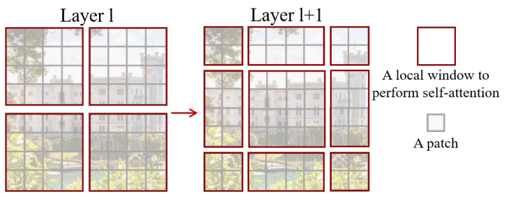[왼쪽] regular window partitioning [오른쪽] shifted window partitioning

Swin Transformer의 또 다른 핵심 구조는 shifted window인데요. 서로 겹치지 않는 window를 사용하는 효율적인 연산 방식은 유지하면서, layer 간 window를 연결하기 위해서 사용하는 구조입니다. 위 그림을 기준으로 설명하면, $l$번째 layer에서는 좌상단부터 시작해서 각각의 window가 $ 4 \times 4 \,(M=4)$개의 패치를 갖도록 $ 2 \times 2 $개의 window로 나눕니다. 그 다음 layer인 $l+1$번째 layer에서는 window가 가로, 세로 방향으로 각각 $\llcorner \frac{M}{2} \lrcorner$만큼 이동합니다. 이렇게 하면 이전 layer의 window간 경계를 포함하는 새로운 window 안에서 self-attention을 수행하게 되므로 layer 간 window를 연결할 수 있습니다.

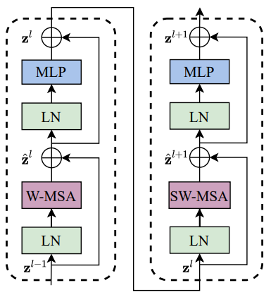
위 그림에서 W-MSA는 regular window 방식으로 multi-head self-attention을 수행하는 것을 의미하고, SW-MSA는 shifted window 방식으로 multi-head self-attention을 수행하는 것을 의미합니다.

3. Relative position bias

self-attention을 계산할 때 아래 수식과 같이 relative position bias $B \in \mathbb{R}^{M^2 \times M^2}$을 추가하고, 학습 과정에서 업데이트 합니다. query, key, value 매트릭스의 차원은 $Q, K, V \in \mathbb{R}^{M^2 \times d}$이므로 $QK^T \in \mathbb{R}^{M^2 \times M^2}$입니다. 이 때, $M$은 window 안 패치의 개수이고, $d$는 query와 key의 차원인데 본 논문에서는 $M=7, \, d=32$를 사용했습니다.

\[Attention(Q,K,V)=softmax(\frac{QK^T}{\sqrt{d}}+B)V\]

실험에 따르면, Vision Transformer처럼 고정된 abolute position embedding보다 relative position bias를 사용하는 것이 더 좋은 성능을 보였다고 합니다. 또한, pre-train 시에 사용한 window와 다른 크기의 window를 fine-tuning 시에 사용하더라도, pre-train 과정에서 학습한 relative position bias에 bi-cubic interpolation을 거쳐서 초기값으로 사용할 수 있습니다.

Experiments

Regular ImageNet-1K training
- Optimizer
  - AdamW optimizer
  - 20 epoch 동안 linear warm-up
  - 300 epoch 동안 cosine decay learning rate scheduler 사용
  - learning rate 초기값은 0.001
- batch size 1024
- weight decay 0.05
Pre-training on ImageNet-22K and fine-tuning on ImageNet-1K
- Pre-training
  - Optimizer
    - AdamW optimizer
    - 5 epoch 동안 linear warm-up
    - 90 epoch 동안 linear decay learning rate scheduler 사용
    - learning rate 초기값은 0.001
  - batch size 4096
  - weight decay 0.01
- Fine-tuning
  - 30 epoch 동안 학습
  - batch size 1024
  - constant learning rate $10^{-5}$
  - weight decay $10^{-8}$

Vision

Transformer Swin-Transformer

This post is licensed under CC BY 4.0 by the author.